Freshness
Monitor data freshness in Validio by tracking the time elapsed since a source was last updated.
Validator Overview
Freshness validators evaluate the time elapsed since the data was last updated on the source. You can backfill data and use segmentation on Freshness validators.
For an overview of all validator types, see Validator Types.
Recommended Setup for Monitoring Freshness
The following setup applies to the majority of use cases for monitoring Freshness:
- Set a daily tumbling window with "Disable Window timeout" checked.
- Set the polling schedule to daily, 1-2 hours after the expected pipeline job completion.
- (Optional) Configure a segmentation field.
Metric Configuration Parameters
| Parameters | Description |
|---|---|
| Filter | (Optional) Select from a list of filters or create a new filter to specify which records to include. |
| Window | Select from a list of windows or create a new window to specify how to aggregate the data. |
| Segmentation | (Optional) Apply segmentation to analyze data in separate groups. Default is Unsegmented. |
Choosing the Window Type
You can only configure Freshness validators to use tumbling or global windows. In general, tumbling windows are recommended whenever possible to enable instant dynamic threshold training and backfill of historic data.
Global windows can be used when you:
- Want to set up freshness validation on a large number of tables and don't need backfill or segmentation on these tables.
- Prefer having the X-axis display the difference for polling time instead of data-time (window end time).
For more information, see About Windows.
Polling and Windows
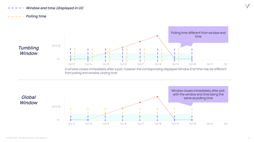
There is a slight nuance to how window end times and polling (how often Validio queries for data) relate to each other, depending on whether you use a tumbling or global window.
- Tumbling window--The window size is set separately from the polling schedule and can be different from each other. The polling schedule can be more frequent, for example every six hours while the window size is daily.
- Global window--The window end time will follow the polling time. For example, if you set the polling schedule to poll every six hours, the window size (x-axis) and window closing time will also be six hours.
For the recommended polling schedule and window configuration, see Recommended Setup for Monitoring Freshness.
In the case of infrequent polling with a small window size, for example if you want to receive incidents on a daily basis but have a 1-hour granularity in your freshness graph: You can set a tumbling window size of 1-hour, with a polling schedule set to daily to save on query costs. Every day at polling time, Validio will backfill 24 1-hour windows from the latest poll.
Setting Window Timeout
For Tumbling windows, you have a "Disable window timeout" option:
| Setting | Option state | Behavior | Use case |
|---|---|---|---|
| Timeout enabled | Unchecked | Allows a grace period of up to 1 window length before closing, depending on if new data has arrived. | Irregular batch updates or continuous data loading where premature window closing is a concern. |
| Timeout disabled | Checked | On each poll, all windows up to the current window will close. | Recommended for most Freshness cases. Regular batch pipelines with predictable schedules. |
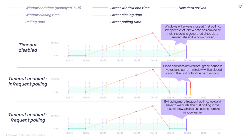
Tumbling window and timeout enabled is primarily used when you expect irregular batch updates, such as when you expect data to sometimes arrive late and you don't want to be alerted each time. In this case, you can poll more frequently than the window size. Another example is when you don't load data in window-sized batches, such as when you have a job that continuously adds new data. In this case, you don't want to disable timeout because then you could close the window prematurely.
Dynamic Threshold for Freshness
Dynamic Threshold uses a dedicated model for freshness validators. The model monitors how long it takes for new data to arrive based on historical arrival patterns and the polling schedule. Each time data is polled, the model observes the window time and creates an expectation of when to expect data next. If the freshness value exceeds the threshold, it is flagged as an incident.
For general information about dynamic thresholds, see Configuring Dynamic Thresholds.
How the Freshness Model Constructs Bounds
Day-of-week seasonality on an hourly window
The model starts by looking for as many patterns in data arrival times as possible. For example, if data is consistently absent on weekends but otherwise fresh, the model will learn not to alert on weekends. It most often takes a few periods for the model to consider incorporating seasonality.
If the model recognizes that stale data is common but occurs randomly, it incorporates that behavior into its prediction. If the overall behavior of your data is deemed unpredictable, the model removes the structure it first imposed and widens its bounds to avoid alerting on what is normal--if inconsistent--behavior.
Seasonality Detection for Freshness
Day-of-week seasonality with an additional fresh datapoint on a Saturday
The freshness model automatically detects and adapts to seasonal patterns in data arrival times. The seasonality level is automatically selected based on historical data and where it is most likely to contribute to model performance.
The model looks for the following seasonality levels:
| Seasonality Level | Period |
|---|---|
| Hour of day | 1 day |
| Day of week | 7 days |
| Week of month | 4 weeks |
| Month of year | 52 weeks |
Early Arrivals
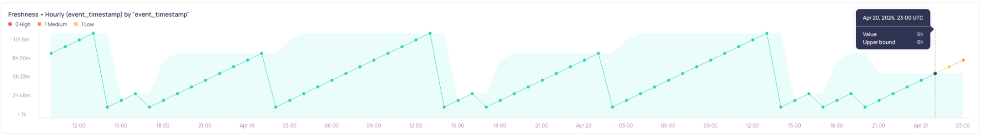
Inserts happen at 00:00, 12:00, and 15:00. On the April 20th, an early arrival at 18:00 breaks the cycle. As a result, the model calculates the time left onto the previous stale period.
When the model has detected a seasonality pattern--for example, data regularly going stale on weekends--a single new data point arriving mid-pattern can interrupt the expected stale period. Because this interruption was caused by one fresh data point, the model does not treat it as a new pattern. Instead, it allows the stale period to continue without triggering an incident. The model then resets its threshold to account for the fact that, while a stale streak would not normally begin at this point in the cycle, the overall seasonal pattern is still intact.
For general information about seasonality detection, see Seasonality Detection.
Decision Bounds for Freshness
Freshness validators default to Upper decision bounds, meaning the model only alerts when data is later than expected. Using Upper bounds also enables the early arrival adaptation functionality described in Seasonality Detection for Freshness.
For general information about decision bounds, see Decision Bounds.
Sensitivity for Freshness
Sensitivity for freshness validators controls how quickly the model alerts when data is late. The freshness model interprets sensitivity presets differently from other validator types:
| Sensitivity Preset | Freshness Behavior |
|---|---|
| Narrow | No extra offset. Alerts as soon as data is late beyond the model's expectation. |
| Default | No extra offset. Alerts as soon as data is late beyond the model's expectation. |
| Wide | Allows data to be one extra window late before alerting. |
Use Wide if it is acceptable for data to be slightly late on occasion. Use Default or Narrow when you want to be alerted as soon as data is late.
Sensitivity change for Freshness: Previously, Default allowed data to be one extra window late and Wide allowed two extra windows late before alerting. Default and Narrow now alert as soon as data is late with no extra offset, and Wide allows one extra window late.
For general information about sensitivity, see Sensitivity.
Model Feedback for Freshness
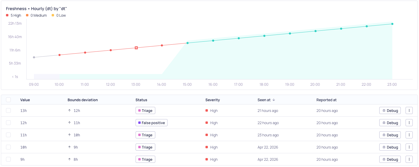
Fasle postive feedback was given at 14:00. The model adapts accordingly and suppresses future alerts for this streak. Once a fresh datapoint arrives, it returns to ordinary operations.
Model feedback for freshness validators is time-aware. Each correction only affects the part of the schedule it applies to. For example, marking a Saturday delay as a false positive will not make the model more lenient on Tuesdays.
When you mark an incident as a false positive, two things happen:
- The current stale data point is immediately accepted. If your data continues to be delayed, the model will stop alerting on this particular delay until fresh data arrives again.
- Future predictions are adjusted. The model remembers that this level of delay is normal for that specific time.
When you mark a missed anomaly as a false negative, the model tightens its expectations at that point in the period, making it more likely to alert on similar delays in the future.
For general information about model feedback, see Model Feedback and Retraining.
Interpreting the Freshness Graph
The time represented in the Freshness graph depends on the window type: data-time for a Tumbling window, and polling time for a Global window.
Freshness with a Tumbling Window
Tumbling windows are configured with a date-time field to represent the data time.
- X-axis--The timestamps on the X-axis represent the end time for each window, using the date-time field. The window end time is based on UTC, but the graph displays the local system time. For example, daily window end times are always 00:00 UTC to 00:00 UTC, and hourly window end times are 01:00 UTC, 02:00 UTC, 03:00 UTC. The window end time is converted to the local system time before it is displayed on the graph.
- Y-axis--The Y-axis displays the difference between window end time and the latest timestamp within the window. Any data containing dates later than the window end time, such as timestamps in the future, will be used in the freshness calculation for the next window.
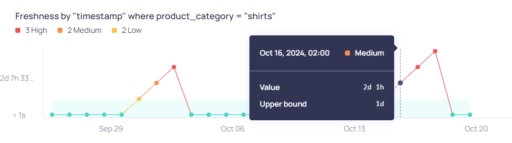
Example
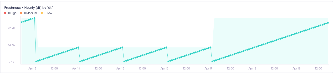
Tumbling window with "screenshot":
- Daily window closed on Oct 16th 00:00 UTC. Oct 16th 02:00 is displayed on the X-axis because the local system time is UTC+2 on the machine where "screenshot" was captured.
- For the window that closed on Oct 16th 02:00 UTC+2, the Y-axis value is 2 days 1 hour, meaning that the latest timestamp that existed in the data at the time of the window closing was Oct 14th 01:00 UTC+2 (Oct 13th 23:00 UTC).
Freshness with a Global Window
Global windows are configured based on the polling time, when the validator checks for new data.
- X-axis--The timestamps on the X-axis represent the local clock-time corresponding to when source polls occur.
- Y-axis--The Y-axis displays the difference between polling time and the latest timestamp in the chosen datetime field.
Updated 3 months ago